Should your system use lock-free data structures?

Discovering the nuance of speed and micro benchmarks

I’ve anecdotally heard over and over that lock free data structures are fast. It’s very hard to get it right, but the performance payoff you can get compared to locking version is lucrative. I have never compared the performance between the two before though, and I thought this would be a perfect topic to learn and write about as my first technical article. So I started writing this article with a conclusion in mind: “Lock free data structures are great! Here’s why it’s awesome”. Maybe this would take me a month or so to test and write about. Boy was I wrong.

This the second version of the introduction I’ve written. In the first version, I went on about how amazing this data structure is, like a shiny new toy I’ve discovered. This quickly fell apart when ran my first benchmark, and this sent me down a rabbit hole about cache coherence protocols, flame graphs, heterogeneous CPU architecture of my M1 mac, and all the headaches of running a reasonable micro benchmark when the measurement is at nano seconds level. So I missed my lofty goal of writing an article per 2 months from my first article already, but I learned a lot and have a lot to share. Hope you’re excited to follow the twist and turns I’ve been through!

---

AI Disclaimer:

This article is entirely written by me. Queue implementations are hand written. AI was used for benchmarking code and visualization code.

---

What is a lock free data structure?

I was introduced to the concept of lock free programming about 2.5 years ago when I was interviewing for my current job. What stood out to me when I was looking at some of the older tech blogs was the lock-free skip list that the memsql engine used. I couldn’t form a good mental model of how it worked back then, quite frankly it was scary to learn that there is a whole different way of dealing with concurrency. Once I started working and started running into these building blocks in the codebase, I felt the necessity to form a firmer mental model of what this paradigm is. Let’s take a line out of Wikipedia:

an algorithm is called non-blocking if failure or suspension of any thread cannot cause failure or suspension of another thread

Think about the typical data structure with a mutex. Before you enter a critical section you acquire a lock, do dangerous stuff, then release the lock. Concurrency 101 which all systems classes teach. This gets us to mutual exclusion, but the system is now at the mercy of the OS scheduler. If the thread is de-scheduled by the OS while holding the lock, then all the other threads can’t acquire that lock cannot make progress, until the original thread comes back again: we have a single point that blocks everyone else.

Lock-free data structures do not have this problem. The mental model that I have is that it reduces the point of logical change of a data structure into a single, atomic CPU operation that nobody has to be blocked on. This means nobody is acquiring anything. There’s nothing to take, no permission to ask for. Your data structure cannot be in a logically inconsistent state where the invariants are broken, not even temporarily. No critical section. That’s pretty cool!

Compare and Swap

We can’t discuss lock-free programming without introducing compare and swap (CAS) operation.

inline bool CAS(Node **ptr, Node *expected, Node *newPtrVal ) {
  return __sync_bool_compare_and_swap(reinterpret_cast<void **>(ptr),
                                      static_cast<void *>(expected),
                                      static_cast<void *>(newPtrVal));
}

bool CAS_expanded(Node **ptr, Node *expected, Node *newPtrVal) {
  if (*ptr == expected) {
    *ptr = newPtrVal;
    return true;
  }
  return false;
}

The CAS_expanded method is what CAS does but in discrete steps. We check if ptr is still storing expected, and if so, swap out what it stores with newPtrVal, all in a single cpu instruction that cannot be interrupted. The common pattern is to design the data structure so that:

1. The data structure can go from one logical state to another by a single pointer swap

2. Set up all the work for the pointer swap, and take a snapshot of the current state of the data structure

3. If the snapshots we took is logically consistent, we attempt to advance the data structure from one state to the other using CAS

4. If it failed, it implies that another thread has advanced the state of the data structure from one to the other in between snapshot taking and CAS attempt. We take a new snapshot and try again until we succeed

This is still theoretical. Let’s take a look at a concrete example.

The Michael & Scott Queue

For the purpose of this article (and the series of follow up articles on lock-free data structures), I’ll be implementing and measuring the Michael and Scott Queue from this paper, which is considered a standard for lock-free queues. We will only be looking at enqueue - once we start involving dequeue and memory management, things start to get weird, and that’s for another day.

It works something like this:

struct Node {
  int val;
  Node *next;
};

class Queue {
public:
  Queue() {
    Node *dummy = new Node();
    head = dummy;
    tail = dummy;
  }
protected:
  Node *head;  // head always points to dummy
  Node *tail;  // insertion always happens at the tail
}

bool LockFreeQueue::enqueue(int val) {
  Node *newNode = new Node();
  if (!newNode) return false;
  newNode->val = val;
  newNode->next = nullptr;

  Node *tailSnap, *nextSnap;
  while (true) {
    tailSnap = tail;
    nextSnap = tailSnap->next;
    if (nextSnap == nullptr) {
      if (CAS(&(tailSnap->next), nextSnap, newNode)) // CAS1
        break;
    } else {
      CAS(&tail, tailSnap, nextSnap);  // CAS2
    }
  }
  CAS(&tail, tailSnap, newNode);  // CAS3
  return true;
}

In Michael and Scott Queue, we have a structure where head is always pointing at a dummy node, and insertion happens only at the tail. Singly linked list with two pointers, logically the first element to be dequeued is head→next→val, head == tail && head→next == nullptr means an empty queue, tail→next is always null, you get the gist.

I’ve annotated the different CAS operations with CAS{1|2|3}. Let’s try to understand this with the steps outlined above in the CAS section.

The data structure can go from one logical state to another by a single pointer swap

The CAS1 is the main insertion point in our queue. We want the tail’s next pointer to point to the new node we just created. We actually need two pointer swaps to make this complete, one for tail’s next to point to the new node, and one for the tail itself to point to the new node. Even without tail not pointing to the new node, the queue is not broken. It can’t be inserted to or the new insertion isn’t visible yet, but it takes one atomic pointer swap to get us out of this state.

Set up all the work for the pointer swap, and take a snapshot of the current state of the data structure

Before we enter the CAS loop, we do all the work for the new node: allocating space, setting up the right values for it to be the new tail, etc.

We then take the snapshot of the queue’s current state. We store the current pointer value of the queue’s tail node, and what that node is pointing to next. Note that for nextSnap, we’re not grabbing tail→next as the tail could have been changed in between tailSnap and nextSnap.

If the snapshots we took is logically consistent, we attempt to advance the data structure from one state to the other using CAS

After taking these snapshots, we’re checking if these make sense in two steps. 1. Is the snapshot of the tail at the end of the queue? 2. At the atomic point of swap, is the snapshotted tail node still at the end of the queue? If answers to both of the questions are yes, CAS succeeds, and the new node we created earlier is now at the end of the linked list. This brings us to the non-insertable-but-not-broken state.

If it failed, it implies that another thread has advanced the state of the data structure from one to the other in between snapshot taking and CAS attempt. We take a new snapshot and try again until we succeed

If CAS failed, this can mean two things. 1. Some other thread inserted a new node between tailSnap and nextSnap, so nextSnap was never null, or 2. Another thread was attempting CAS at the same time as this thread, and won out. In MS Queue, we simply retry by starting with the snapshot taking again, until we succeed.

The resolution of going from non-insertable-but-not-broken state to a good state happens in CAS2 and CAS3. Borrowing from the terminology from the paper, these are added so that we “swing” the tail pointer to the newly inserted node. We attempt this in both the thread that inserted the node (CAS3) and the thread that observed this non-insertable state (CAS2) to guarantee that no matter what thread you are, you can make progress on your own.

So what does this mean in real workload?

We get nice guarantees that are otherwise impossible on a traditional mutex-based queues. But how does this perform under real life workloads? Consider a simple insertion workflow. Spin up multiple threads, let each threads call enqueue certain amount of times, and measure the throughput. What do you think will happen as we increase the number of threads and increase the odds of contention?

Context switching is expensive. Every switch involves dumping the CPU & register state and reloading a different context that piles up. More often we need to switch, the worse. In mutex version, some threads can’t make progress if the lock is held by another thread and is forced to yield/trigger a context switch before making progress. Compare this to a lock-free queue that doesn’t need his overhead. My intuition was that the lock-free queue will blow away the mutex queue on throughput as the number of threads scale for this reason.

How does lock-free queue perform?

The first benchmark

With the lock-free implementation and mutex implementation (code omitted) ready, I was ready to benchmark parallel enqueue scenario. Here’s the setup:

1. Enqueue 10M elements into the queue, elements are split up evenly across N number of threads

2. All threads are sequentially calling enqueues

3. Repeat this workload 5 times, and calculate the throughput

4. Start from N=1 to N=32

5. This benchmark is run on my 2021 Macbook Pro with 8 cores, compiled with -O2

Fig 1. Insertion throughput from 1 thread to 32 concurrent threads

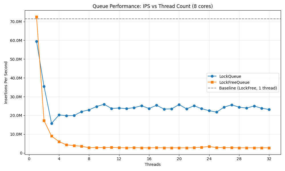
…wait what?

The lock-free queue was performing noticeably worse as I scaled the number of threads. Notice how the performance falls off a cliff as soon as we add another thread in the mix. At this point I started scrambling. I was supposed to write about why lock-free queues are fast! For good measure I ran the same benchmark with 10k - 100k threads with 10k threads step.

Fig 2. Insertion throughput from 10k threads to 100k concurrent threads

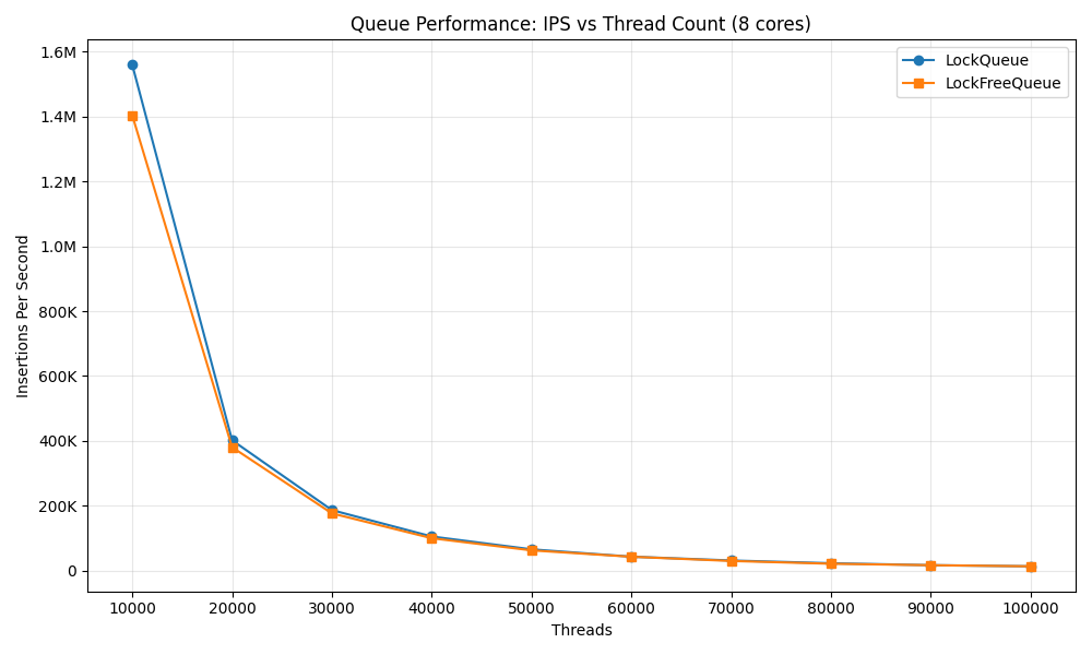
Of course, running this many threads is non-sensical in practical sense, but the story is the same. As the number of threads scale both implementation slows down which makes sense it means more contention, but the performance of the lock-free implementation never overtakes the mutex based implementation. At this point I was doubting my own implementation. Did I implement the Michael Scott queue wrong?

Fig 3. Insertion throughput from 1 thread to 32 threads, my own queue implementations and xenium lib

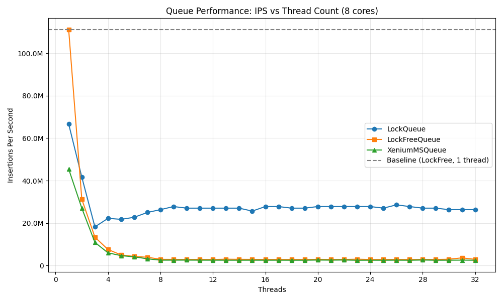
Not really. I tested both implementations against an existing implementation of the same paper in xenium lib, and the performance numbers of the library implementation and my own implementation were more or less the same. This didn’t match my intuition, and I was determined to understand what kind of gap I had in my understanding of lock-free programming.

Understanding the bottleneck through Flame Graphs

The next natural step is to see where exactly are we spending the most time in the lock-free queue implementation. The tool for this is FlameGraph. For those who are unfamiliar, it’s an open source visualization tool for understanding where the CPU is spending the most time in the stack trace. I hooked it up to my lock-free implementation and gave it a go with 8 concurrent threads.

Fig 4. FlameGraph for lock-free queue

Fig 5. FlameGraph for mutex queue

This paints an interesting picture. What stands out in the lock-free version is that about 50% of enqueue time is spent on CAS2. What does this mean? Let’s look back at the CAS loop snippet again:

tailSnap = tail;
nextSnap = tailSnap->next;
if (nextSnap == nullptr) {
  if (CAS(&(tailSnap->next), nextSnap, newNode)) // CAS1
    break;
} else {
  CAS(&tail, tailSnap, nextSnap);  // CAS2
}

A thread takes CAS2 path if some other thread succeeded in CAS1 and no-one else have swung the tail to the new node successfully yet, either through CAS2 or CAS3. The fact that near majority of the time is spent here is alarming. Let’s paint this picture: 8 threads all running on 8 cores trying to enqueue simultaneously. One of them succeeds in CAS1. Other 7 threads now either fail CAS1 or hit CAS2, and retry. This happens continuously: only one thread is doing proper work and others are continuously burning the CPU cycle retrying.

Compare this to the mutex version. Majority of the time spent here are in psynch_mutexwait, where the threads that failed to acquire the lock are sleeping. With 8 threads running concurrently, the thread that won will continue to enqueue un-interrupted while other 7 are sleeping, waiting for their turn, so CPU cycle isn’t burned here.

What I suspect that makes it worse for lock-free implementation is cache coherence protocol coming in the mix. All threads are trying to read and write to the same memory address to swing the tail, without sleeping. Every successful write will trigger synchronization on the cache line across all cores, invalidating everyone else’s cache line containing the tail, and forcing them to re-fetch the cache line… continuously! This is cache thrashing. Mutex version doesn’t suffer from this given other threads are sleeping, so things can stay in L1 cache for much much longer. I don’t have a direct evidence of the above, but I plan on diving deeper into cache coherence protocols in future blogs. Perhaps I can revisit validating this theory then.

First benchmark post mortem

This experiment was a fun wakeup call. Lock-free data structure is not a drop-in replacement for the mutex counter part that magically gives performance gain. My naive expectation was that since the system guarantees independent progress, this vaguely translates to higher throughput under high concurrency. The reality is that these two data structures have very different performance characteristics, not one being the superset of the other.

In hindsight, the benchmark itself is not designed to highlight the benefit of lock-free queue either. There’s a single point of insertion no matter how many threads you throw at it, and there’s no sleep between these insertions. As long as some thread is running, enqueue will continue to happen in a serializable way in a tight loop for both queues. Every thread is competing with each other and we’re just measuring the overhead at this point. What this benchmark has shown is that this overhead can be very high for the lock-free queue when the contention is high, caused by cache thrashing.

I needed to find a different way to demonstrate why of lock-free queues and understand under which workload patterns this works well. Let’s rethink the benchmark design.

How does lock-free queue really perform?

The second benchmark

I want to design a scenario that is much more favorable to lock-free queues. Mutex-based queue’s worst case performance is when the thread that is holding the lock is preempted - other threads are blocked and system can’t make progress until the holder is scheduled again. This problem gets worse as the number of threads scale: more threads means less opportunity for the lock-holder to come back. There may be more nuance on how the kernel decides to schedule a thread, but let’s work with a simple model for now.

I expect that this will translate to worse tail latency. Thread preemption while holding a lock is a probabilistic and unpredictable event, and when this happens all threads experience a latency spike. This can be unacceptable in certain systems where it needs the distribution of latency to be tight and predictable. So, let’s try to design a benchmark that dramatizes this effect.

1. Using similar workload as the first benchmark of parallel insertion, but now both queues have 0.05% probability of sleeping for 1us to 1ms. For mutex queue, this happens at the critical section. For lock-free queue, this happens right before the insertion CAS (CAS1).

2. We will measure how long individual enqueue took and store it in a long vector

3. We will make a box plot for the latency distribution, measuring avg, p25, median, p75, p99 and p99.9

It’s worth pointing out that this is a very engineered benchmark. Injecting probabilistic sleep like this is just modeling pre-emption since controlling this behavior is quite difficult (I’m not sure if it’s even possible).

Microbenchmarking is hard

Before I share the results, I want to reflect on unexpected results I ran into while working on this second benchmark. Now that I am measuring the individual enqueue speed rather than the throughput of the system. There were more details I had to be aware of at a lower level. I want to share some of these gotcha moments.

Coincidentally I’m drinking microbench coffee from terminal.shop as I’m writing this (not sponsored), one day @theprimeagen will notice me

Time measurement granularity

As I started getting initial version of the plot, I noticed that a lot of measurements were in 0ns, 41-42ns, and some multiple of 42ns. The measurement code used c++ chrono library, nothing special.

auto tStart = std::chrono::steady_clock::now();
q->enqueue(val);
auto tEnd = std::chrono::steady_clock::now();
long ns = std::chrono::duration_cast<std::chrono::nanoseconds>(tEnd - tStart).count();

The secret lies in the timebase of the machine I’m running this in. std::chrono::steady_clock depends on the monotonically increasing counter of my laptop, which is dependent on the frequency of the hardware clock. We can observe this easily:

$ sysctl hw.tbfrequency
hw.tbfrequency: 24000000

Given that my mac’s hardware clock runs at 24MHz, this means an individual tick is 1s / 24MHz that is equivalent to 41.667ns. It’s impossible for me to measure below this granularity at least on this machine. 0ns doesn’t mean it actually took 0ns to enqueue, but rather it took less than 41ns, and the clock tick hasn’t happened between the measurements. On top of this, the act of measuring the current time itself is an overhead that’s non-negligible. Keep this in mind as you see the numbers.

Heterogeneous CPU architecture of M1 Mac

I was looking at the performance numbers when the workload had 1 thread vs 8 threads. What surprised me was that the median enqueue time was 5x more when we were running with 1 thread vs 8 threads. This was unintuitive: we’ve already established the overall throughput falls as number of threads scale due to contention. Shouldn’t the median enqueue time stay stable or get worse as we add more threads?

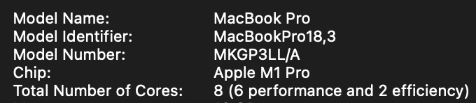
Notice the detailed spec of this mac. Notice that among the 8 cores, 6 are “performance” and 2 are “efficiency”. M1 Mac chooses an asymmetric multiprocessing architecture that uses different type of cores for battery efficiency. The background jobs that doesn’t need to be performance will be placed on the efficiency core for example. This doesn’t work well for our microbenchmarking - if the enqueue thread in 1 thread benchmark is pinned to the efficiency core, that doesn’t make for a fair comparison. Thankfully we can specify the priority of the worker thread by specifying the Quality of Service (QoS) and force it to run on the performance cores.

pthread_set_qos_class_self_np(QOS_CLASS_USER_INTERACTIVE, 0);

After setting this, I finally started seeing sane performance number between 1 thread vs 8 threads benchmark.

Predictable system that scales

With these adjustments, I was able to observe how lock-free queue’s enqueue latency distribution looks like, and how it compares to mutex queue.

Fig 6. Enqueue latency distribution for single thread worker

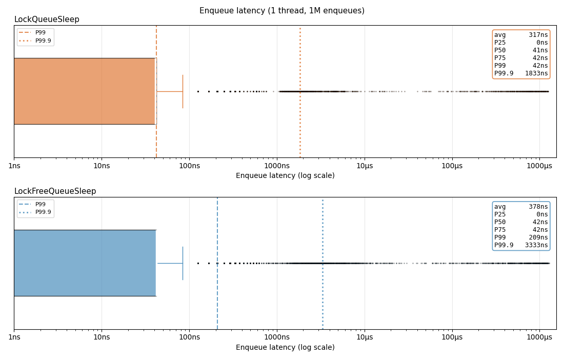
Both queues have very comparable numbers, with lock-free queue performing slightly worse. Still, the majority of the enqueues happen within a two clock ticks for both implementation.

Fig 7. Enqueue latency distribution for 8 worker threads

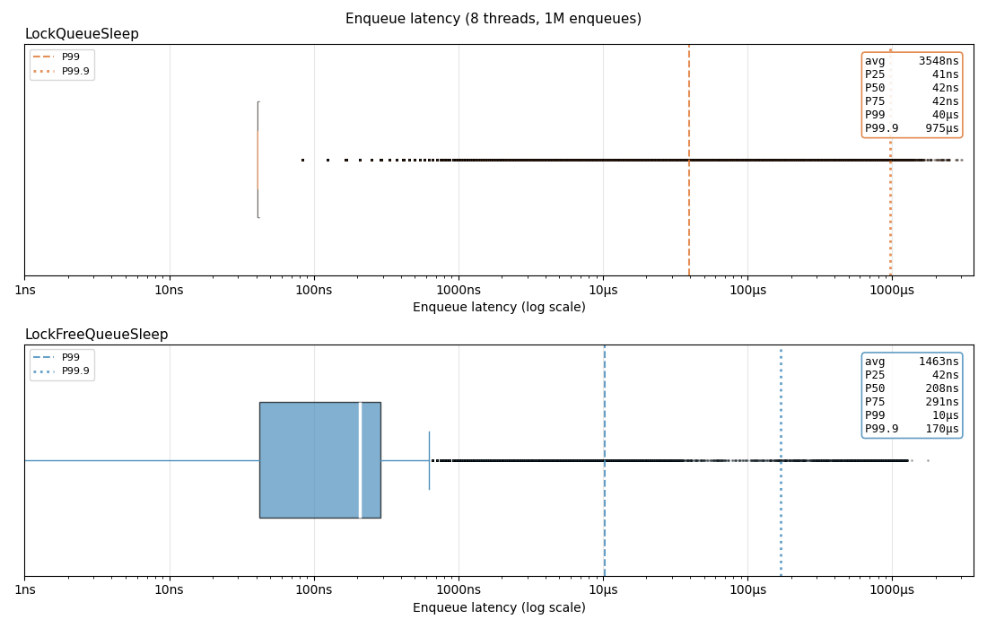
This distribution changes dramatically when we have 8 worker threads. p75 numbers are comparable and doesn’t change much for mutex queue, and lock-free queue sees some performance degradation from contention and cache thrashing. What is noticeable is how the tail latency (p99 and p99.9) for mutex queue is 4~7x worse than the lock-free queue, almost approaching 1ms.

Fig 8. Enqueue tail latency scaling

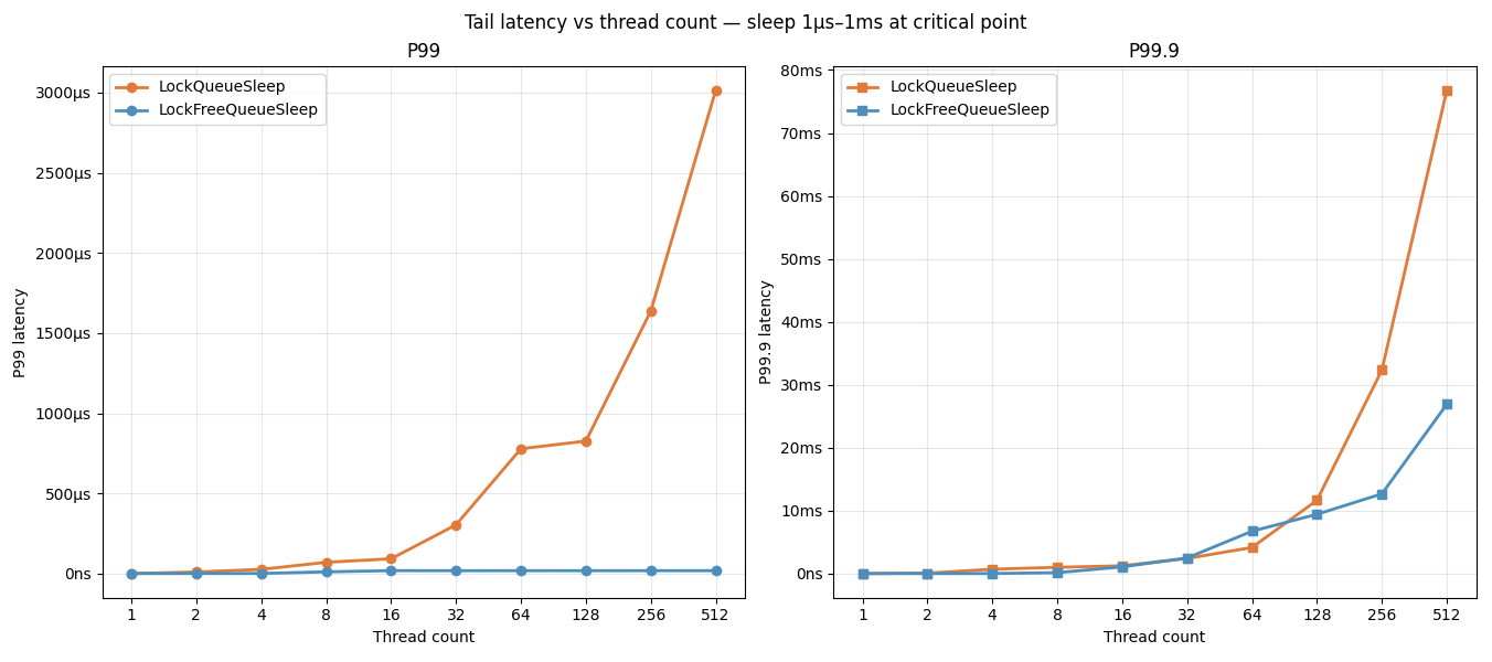
We can keep increasing the thread count and see how the tail latency scales for both implementation. Notice how the more threads we add, the mutex queue’s tail latency scales badly, compared to lock-free queue that shows a more or less stable or slower scaling curve. This is scalability that we can see clearly. As we expected, the mutex based queue’s tail latency degrades very fast, but the lock-free queue is able to keep the distribution much tighter.

The Takeaway

So, coming back to the original question in the article, should your system use lock-free queues? It depends. We observed that using lock-free queues sacrifices average case throughput in favor of tail latency scalability. Lock-free data structure comes with clear tradeoffs. The complexity introduced to the codebase, and the average performance that can be worse. Most applications can get away and be perfectly fine with a mutex-based data structure. But if your systems runs under very high concurrency and need certain latency distribution requirements, then lock-free data structure can be a very reasonable choice.

If you are thinking of using lock-free data structures, you should measure it. The performance characteristics will change drastically based on the workload pattern of the application, and it’s impossible to make a generalized statement. Modern computer architecture adds another layer of complexity that can deviate the expectation from reality. As system developers, the best we can do is to acknowledge the unknowns, measure, what are the requirements of the system, and understand the tradeoffs we’re making by these design choices.

Looking into the future

I had lot of fun writing this, and hope you had did too following this along. I’m glad I got to sit down and observe how these fundamental layers behave in different scenarios, and learned something new long the way. I want to write more articles like this in the future, exploring things such as cache coherence protocols, dequeue side of the lock-free queue, and other system topics. If you have any suggestions or comments on the benchmark & learnings I’ve done in this article, please let me know in the comments!

---